MARGINAL PROPENSITY TO SAVE.......FACTS AT HANDS

               Marginal propensity to save

The marginal propensity to save (MPS) refers to the increase in saving (non-purchase of current goods and services) that results from an increase in income i.e. The marginal propensity to save might be defined as the proportion of each additional dollar of household income that is used for saving. It is also used as an alternative term for the slope of the saving line.^[1] For example, if a household earns one extra dollar, and the marginal propensity to save is 0.35, then of that dollar, the household will spend 65 cents and save 35 cents. It can also go the other way, referring to the decrease in saving that results from a decrease in income.
The MPS plays a central role in Keynesian economics as it quantifies the saving-income relation, which is the flip side of the consumption-income relation, and thus it reflects the fundamental psychological law. Marginal Propensity to Save is also a key variable in determining the value of the multiplier.

                                Calculation of MPS

MPS can be calculated as the change in savings divided by the change in income.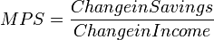

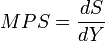Or mathematically, the marginal propensity to save (MPS) function is expressed as the derivative of the savings (S) function with respect to disposable income (Y).

where, dS=Change in Savings and dY=Change in income.

                             An example

	Savings	Income
A	200	1000
B	400	1500

Now, MPS can be calculated as follows:

Change in savings = (400-200) = 200

Change in income = (1500-1000) = 500

MPS = (Change in savings) / (Change in income)

so, MPS = 200/500 = 0.4

This implies that for each additional one unit of income, the savings increase by 0.4.
There are different implications of this above-mentioned formula.

• First it quantifies induced savings.Induced saving is the portion of saving that responds to changes in income^[2].In other words, induced saving can be defined as the household saving that depends on income or production (especially disposable income, national income, or even gross domestic product).^[3]

• Second, it is a measure of slope of the savings function.

                                        Value of MPS

Since MPS is measured as ratio of change in savings to change in income, its value lies between 0 and 1.^[4] Also, marginal propensity to save is opposite of marginal propensity to consume.
Mathematically, In a closed economy, MPS + MPC = 1^[5][6]since an increase in one unit of income will be either consumed or saved.
In the above example, If MPS = 0.4, then MPC = 1 - 0.4 = 0.6.
Generally, it is assumed that value of marginal propensity to save for the richer is more than the marginal propensity to save for the poorer. If income increases for both parties by $1, then the propensity to save for a richer person would be more than that for the poorer person.^[7]

                 Slope of Saving line

Marginal propensity to save is also used as an alternative term for slope of saving line. The slope of a saving line is given by the equation S = -a + (1-b)Y^[8][9], where -a refers to autonomous savings and (1-b) refers to marginal propensity to save (here b refers to marginal propensity to consume but as MPC + MPS = 1, so (1-b) refers to MPS).
In this diagram, the savings function is an increasing function of disposable income i.e. savings increase as income increases.^[10]

The savings function

                         Multiplier effect

An important implication of Marginal Propensity to Save is measurement of the multiplier. A multiplier measures the magnified change in aggregate product i.e. the gross domestic product, resulting from a change in an autonomous variable (for example, government expenditure,investment expenditures,etc.).
The effect of a change in production creates a multiplied impact because it creates income which further creates consumption. However, the resulting consumption is also an expenditure which thus, generates more income, which creates more consumption. This next round of consumption leads to a further change in production, which generates even more income, and which induces even more consumption.
And thus,as it goes on and on, it results in a magnified, multiplied change in aggregate production initially triggered by a change in autonomous variable, but amplified by the creation of more income and increase in consumption.

                                Mathematical implication

Mathematically, the above effect can be stated as:

• In round 1, there is a change in an autonomous variable (say the government invests in a bridge making project for which it approaches a construction company) by an amount $1 (just an assumption for simplification). Now let the marginal propensity to consume for the construction company be 'c'. Thus, the construction company would spend an amount c×$1 i.e. $c.
• In round 2, the construction company incurs expenditure ($c) by procuring raw materials, say cement,steel,gravel,mortar,etc. from respective companies and thus, this amount $c becomes income for these companies. Now again the marginal propensity to consume for these companies is same as the construction company at 'c' and thus, their consumption becomes c×$c i.e. $c².

And it goes on and on. We can express this as:

Round	Change in income	Amount consumed
Round 1	$1	$c
Round 2	$c	$c2
Round 3	$c2	$c3

And so on...

Thus, total magnified change in production due to change in an autonomous variable by $1

= 1 + c + c2 + .................(infinite series)

= 

= 

                              Measuring the multiplier

The effect of a multiplier effect can be measured as: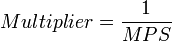

If the MPS is smaller, then the multiplier process is also greater as less saving is induced, and more consumption is induced with each round of activity.^[11]
For example, if MPS = 0.2, then multiplier effect is 5, and if MPS = 0.4, then the multiplier effect is 2.5. Thus, we can see that a higher propensity to save implies a lower multiplier effect and vice-versa.

                                Footnotes

1. ^ Blanchard, O. (2006). Macroeconomics. (Fourth ed., p. 59). Pearson Education Inc.
2. ^ Robert Marks, "Macroeconomics for manager" ,Lecture Series,March 1997,Australian Graduate School of Management, University of New South Wales
3. ^ "Induced Savings", AmosWEB LLC,Economic WEB*pedia,2010-2011.[Accessed: November 8,2011] Web.
4. ^ Blanchard, O. (2006). Macroeconomics. (Fourth ed., p. 59). Pearson Education Inc.
5. ^ Chamberlin, G., & Yeuh, L. (2006). Macroeconomics. (p. 23). Italy: Thomson Learning Inc.
6. ^ Ahuja, H. L. (2008). Macroeconomics : Theories and policies. (14th ed., pp. 125-126). Delhi: S.Chand and Co. Ltd.
7. ^ Carroll, C. (2000) Why do the rich save so much, in Does Atlas Shrug? Economic Consequences of Taxing the Rich, Slemrod, J. (Ed.), Cambridge University Press, London.
8. ^ Froyan, R. T. (2005). Macroeconomics : Theories and policies. (Eighth ed., p. 123,130). Pearson Education Inc. Pvt. Ltd. and Dorling Kindersley Publishing Inc.
9. ^ Dwivedi, D. N. (2005). Macroeconomics: Theory and policy. (2nd ed., p. 73). New York: Tata McGraw-Hill Publishing Co. Ltd.
10. ^ Dornbusch, R., Fischer, S., & Startz, R. (2004). Macroeconomics. (Ninth ed., pp. 217,221-23). New York: Tata McGraw-Hill Publishing Co. Ltd.
11. ^ Chamberlin, G., & Yeuh, L. (2006). Macroeconomics. (p. 23). Italy: Thomson Learning Inc.